
Parallel Python on a GPU with OpenCL
06 Sep 2014Run code on the what?
I had a Wordpress blog in a previous life but I deleted it the other day, right after I made this site. I had only one post on that blog that attracted any attention. At the time I was a student working with time-series data obtained from various telescopes in Sutherland, in South Africa. Some of these datasets were rather a bit larger than I was used to at the time and the running times of some of my programs was slightly obscene.
Then I received a QUAD CORE machine to use at the Observatory. It was great! I thought I’m going to write the worlds fastest parallel code and everything will be awesome. Turns out writing parallel code is hard. Really hard. I also learned that Python can basically not do parallel computations (or so I thought, Global Interpreter Lock what?)
Being an astronomy student, I was exposed to Fortran. And not the ‘nice’ Fortran 95, nope, the old kind with no code in the first 6 columns and everything in CAPS and variable names shorter than 6 characters O_o One gets used to that stuff and once you do you can write some fairly understandable stuff that runs like greased lightning. But you don’t really want to if you know Python. So I learned the concept of profiling my code and rewriting only the slow parts in a compiled language and it is during this time that I figured out not only how to call Fortran code from Python, but also how to use OpenMP to parallelize it. I wrote what I learned on that old Wordpress site and that was the only one that got any attention from the outside world, and not a lot of it. Now it just so happens that I learned something new again. I’m not a student anymore and I don’t get to work with science data nearly as much as I would have liked to but I still like tinkering with computers and writing code.
I learned how to take that code that takes too long to run, even if you run it on 8 threads on an overclocked i7, and make it run on 1000+ cores on a graphics card. Yep.
Let’s make something then make it fast.
So the idea is to show a simple calculation that is easily done in just a few lines of python+numpy and then show how much faster (or slower) that code runs if you go through the effort of redoing it in another language or using another tool.
The one thing I used a lot was the Deeming periodogram. It is basically a Discrete Fourier Transform [DFT]. In astronomy it is used to find periodic signals in time-series datasets and this is exactly what I used it for. I just got bored with waiting for my computer to finish calculating them for me.
Wait, you calculated the DFT from its definition? Why not a Fast Fourier Transform (FFT)?
Here’s the problem. The FFT algorithm assumes that the samples are regularly spaced (in time, say) and the DFT doesn’t make this assumption and in astronomy the observations are almost NEVER done exactly N seconds apart. So I had to use the slow algorithm OR I had resample the dataset into one that was evenly sampled in time. I chose the former because thats what was done by everyone else (maybe a topic for another post).
OK, so here’s what the Python code looks like for calculating a Deeming Periodogram:
def periodogram_numpy(t, m, freqs):
    ''' Calculate the Deeming periodogram using numpy
    '''
    amps = np.zeros(freqs.size, dtype='float')
    for i, f in enumerate(freqs):
        real = (m*np.cos(2*np.pi*f*t)).sum()
        imag = (m*np.sin(2*np.pi*f*t)).sum()
        amps[i] = real**2 + imag**2

    amps = 2.0*np.sqrt(amps)/t.size
    return amps
It’s super simple and for small amounts of data it runs in less than a second and that’s all fine. Simple is good and fast enough is good. But I didn’t always have small amounts of data. I also had an extra complication that has to do with the mathematics of Fourier Transforms. In the above code you can see that there is one loop that runs in Python and it loops over all the frequencies given. There is another loop inside that but you don’t see it in this code because it runs inside of numpy behind the scenes. The invisible loop runs over every data point. So this function touches every frequency once, and for every frequency, it touches every data point. So the number of operations can be estimated by multiplying those two together i.e.:
Operations = Nfrequencies × Mdata points
There’s a couple more operations hidden away in there but we’ll ignore them for now. That number can climb quite rapidly and this kind of algorithm is said to have O(N²) (of the Order N×N) complexity. So the more data you have the longer (and then some) it takes to do. So how do you make it go faster? The correct answer is: DO LESS, which really means, in computer science terms, to choose an algorithm that can do what you want to do, in fewer operations. Sometimes this is just not a possibility and even after selecting the best algorithm you still have so much calculations that you can go to the bar for a few hours while your computer sits and chugs away at the numbers. (Hey why optimize at all?)
One thing to notice is that this algorithm can be done in parallel. You do not need to know the result from the previous frequency bin to obtain the next one, in this instance. So nothing stops you from calculating all the frequency loops simultaneously. This is where my old blog post came in and where this one starts and takes it a bit further. We are going to do those loops in parallel and we are going to use a time-tested language (because I wrote the code long ago and it still works and I’m too lazy to do it in a modern language again).
Requirements for the code
I have a Gist that contains the code I ran to get all the results. You can
find it here. It contains a script
(build_deeming.sh) that will build the necessary things and another
(deeming.py) that runs the whole benchmark. I’ve updated the script to work
with Python 3.4, it should run on python 2.7 too. Let me know if you’d like a
pip requirements.txt file for easy dependency installations. You’ll need at least the following:
pip install numpy matplotlib cython pyopencl
as well as a c and fortran compiler. I used gcc and gfortran. You’ll
also need a working opencl installation. I’m unsure as to what that entails
but I HAVE installed the entire CUDA SDK, Nvidia drivers as well as pyopencl.
The Results
OK on to the fun stuff!
When deeming.py is run, it will compile the opencl kernel and the cython
versions the first time you run it, after that they are cached will just be
called. It will then proceed to calculate the deeming periodograms for 1000,
2000, 4000, 8000, 16000, 32000 and 64000 datapoints and frequencies. This takes
a good few minutes to complete on my computer. I have the following goodies:
- 64 Bit Manjaro (Arch) Linux
- Intel Core i7-920 @ 3.6GHz
- 8GB RAM @ 1333MHz
- NVidia Geforce 760 GTX 2GB
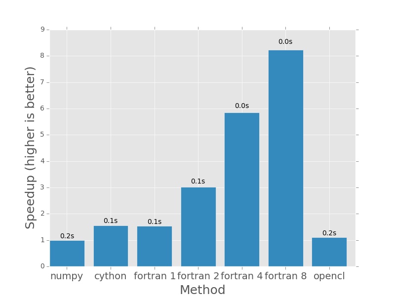
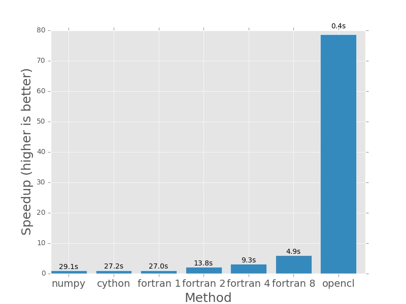
Here are the plots that are produced by deeming.py. The bars represent how
much faster each method is than the numpy version I posted earlier in the post.
In each case the numpy version will have a speedup of exactly 1.0. I plotted
the actual execution time in seconds on top of every bar. In the case of the
Fortran version (which is parallelised with openmp), the number next to the name
denotes the number of threads that was used in the calculation.
First up, 1000×1000. Nothing much to see here. For small amounts of data it won’t take long to complete.
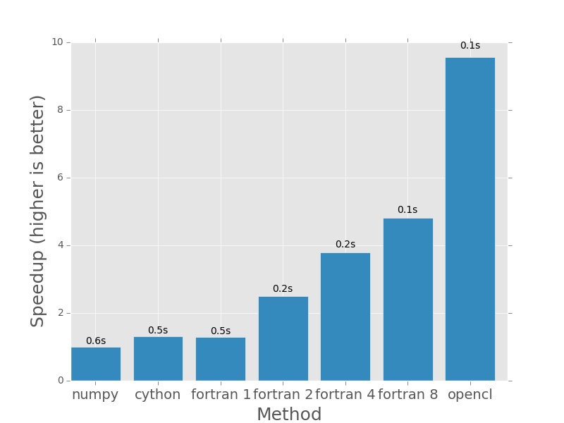
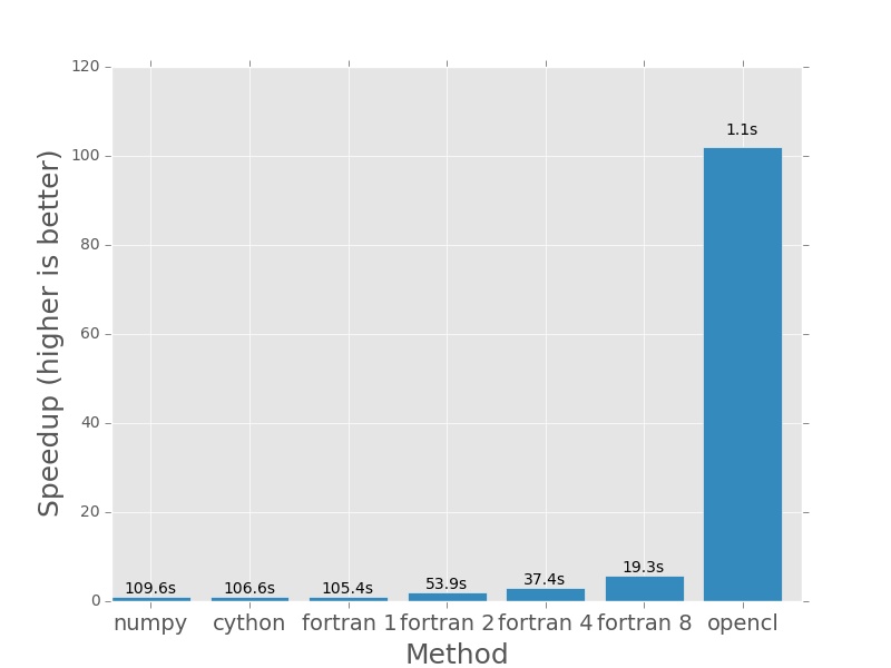
Next up 2000×2000, everything still pretty fast.
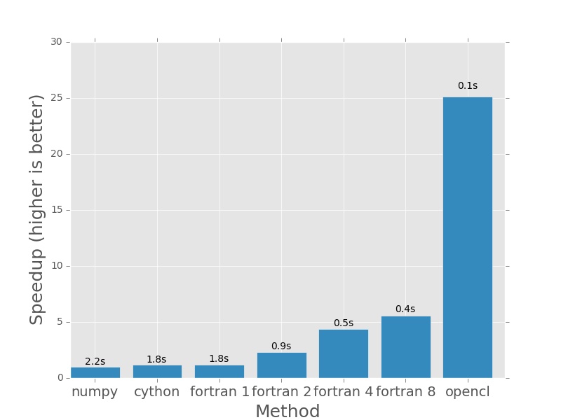
And from here onwards, things get silly. The 760 is starting to show its muscle.
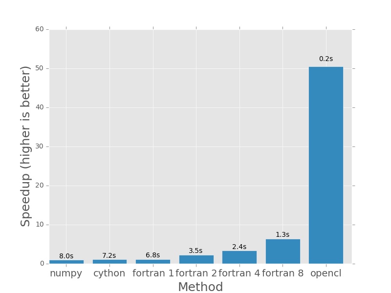
For 64000×64000 operations, even the multithreaded fortran code takes minutes to complete and the GPU is hardly breaking a sweat, completing the calculation in less than 120th the time it takes the single threaded versions to do it and almost 25 times faster than even the 8 thread Fortran version!
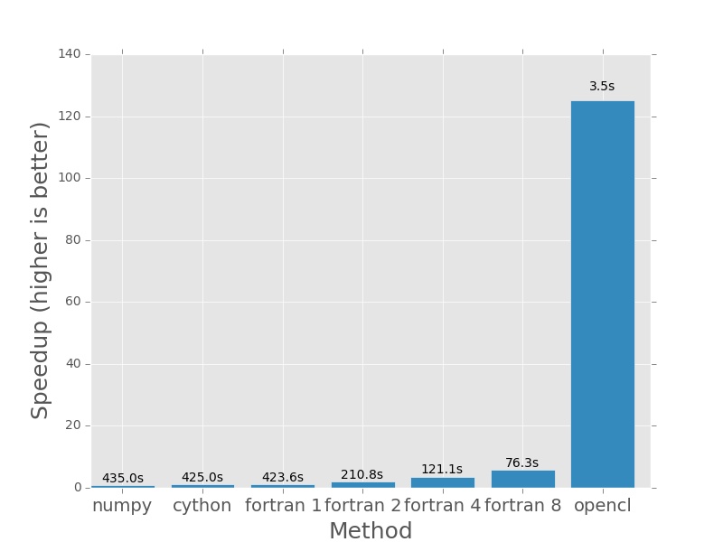
The code needed to do this was not super hard to write but it wasn’t as easy as the original numpy version was and while this increase in performance is astonishing, most real-world applications won’t see these kinds of results due to Amdahl’s Law. I still think it is astonishing that I could make my numpy function go 120x faster with 6 times the amount of code (and a light sprinkling of 1152 cores).
I hope this helps someone. Please leave a comment!