Playing with Photogrammetry 3: Finding targets

• The story so far…
• Contours!
• Ellipses: I have too many
• Selecting the targets
  • Measuring the encoding of a target
• Putting it all together!

The story so far…

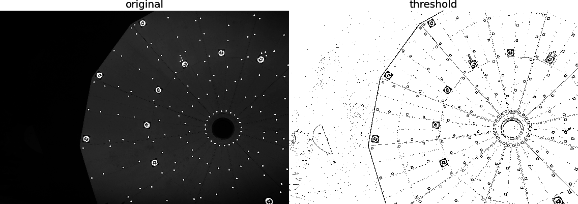
In the previous post I discussed how it is possible to find areas of interest on images like I got from my friend. I showed how one can use an adaptive threshold technique to transform your image into one that only has image values of 0 or 255. Here are our before and after images:

Let’s see a closeup of a target on the threshold image again (from the last post):

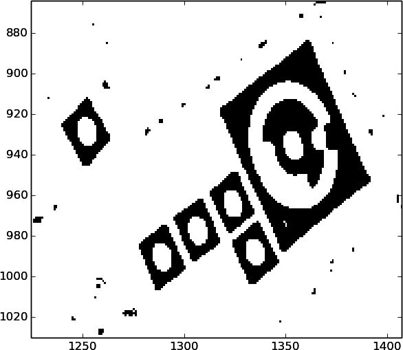
The next thing I needed to do was to find the regions where the targets are located. The threshold image is perfect for this because it only has regions that is one of two values.

Contours!

The reason the threshold image is great is because if I calculate contours of the image values, the contours will fall exactly on the boundaries between the light and dark parts of the targets. This way I get to leverage a powerful algorithm that will give me a much smaller amount of data to work with as well as polygons which are situated near the regions I’m interested in.

From Wikipedia:

“More generally, a contour line for a function of two variables is a curve connecting points where the function has the same particular value.”

opencv has a function that can calculate the contours for me. I used it in the following way:

def get_contours(self):
    ''' Get contours in given image'''
    threshold = copy.deepcopy(self.threshold)
    contours, hierarchy = \
        cv2.findContours(threshold,
        cv2.RETR_TREE,
        cv2.CHAIN_APPROX_SIMPLE)
    # filter out short ones
    contours = [cnt for cnt in contours if len(cnt) > 10]
    return contours

The line containing copy.deepcopy is to avoid my threshold image being destroyed by the contouring function. That line makes a completely separate copy of the threshold, which I don’t mind being mangled by another function.

The last bit is a python list comprehension that filters out contours that is shorter than 10 vertices.

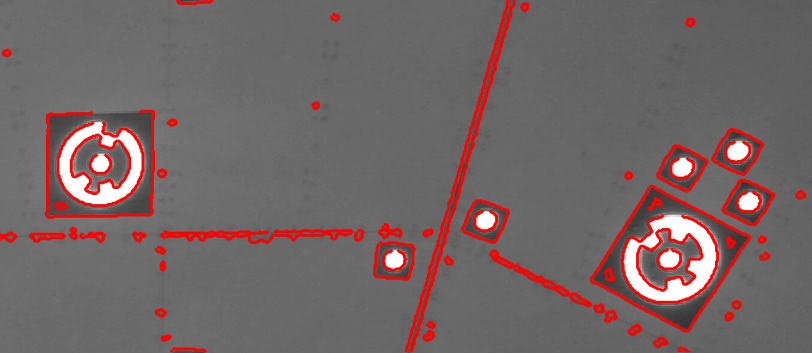
Plotting the contours over the original image gives us something like this:

The contour function returns a list of contours and these in turn are basically lists of the coordinates of the contours’ vertices. I know I wanted the positions of the targets (this is what I’m trying to do, after all). There are a few ways I could do this:

• calculate the centre of mass of the contour vertices
• fit an ellipse to the contour coordinates and use its centre

I rejected the first option immediately because many of the contours are asymmetric. I really want the centre of ellipses and the contours are just rough estimations of where I may find an elliptical target.

The second option works but it is not ideal. For the contours that are located on the outer edge of a RAD target, there is a concave part where the notch is. If I blindly fit an ellipse to these contours, that concave part will skew the ellipse’s centre along a line from the notch through the centre. The ellipse’s values will also be affected. In the image below I illustrate this problem.

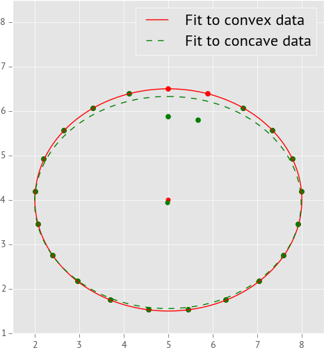
In the plot ¹, the red markers show data points where the edge of an ellipse falls. In the case of the red markers, all the points fall on the edge of some ellipse (I know this because I made up the numbers). In the case of the green points, I changed two of them to fall on the edge of a smaller ellipse that is otherwise the same as the one we have here. This simulates the zero-notch we get on the outer edge of the RAD targets.

I calculated the best-fitting ellipse for each dataset and I plotted those ellipses over the data points. The ellipse fitted to the convex points (no notch) is a solid (red) line and the ellipse fitted to the points containing the notch is a dashed (green) line. I also plotted the centres of both ellipses. As you can clearly see, the two ellipses are not the same and the two centres are also slightly offset.

The way I got around this was to find a way to ‘get rid’ of the notch. What I needed was a polygon that would fit around the contour (notch and all) but bridge that gap where the notch is. Sound familiar? Again, luckily, this is a solved problem. Enter the convex hull.

From Wikipedia:

In mathematics, the convex hull or convex envelope of a set X of points in the Euclidean plane or Euclidean space is the smallest convex set that contains X. For instance, when X is a bounded subset of the plane, the convex hull may be visualized as the shape formed by a rubber band stretched around X.

A rubber band stretched around X eh? Now the cool thing is, the convex hull calculation will not add any new data points to my ellipse contours. It will give me straight lines between points that are already on my ellipses, should it encounter a notch or concave segment. This way, if I fit an ellipse to the convex hull points, the notchy parts do not affect my fits so much and hence I get very good coordinates for the centers of the ellipses.

So, armed with this knowledge I set out to calculate, for each contour I got from the threshold, the convex hull. It is to this that I fitted ellipses.

Ellipses: I have too many

I went ahead and fitted an ellipse to the convex hull of every contour. Again, I utilised the opencv function for fitting ellipses to the convex hulls:

def _find_ellipses(self):
    ''' finds all the ellipses in the image
    '''
    ellipses = []
    hulls = []
    # for each contour, fit an ellipse
    for i, cnt in enumerate(self.contours):
        # get convex hull of contour
        hull = cv2.convexHull(cnt, returnPoints=True)

        if len(hull) > 5:
            ellipse = cv2.fitEllipse(np.array(hull))
            ellipses.append(ellipse)
            hulls.append(hulls)

    return ellipses, hulls

Note that I offhand discarded contours for which the convex hull contained fewer than 5 vertices, the target convex hulls are a bit larger than that.

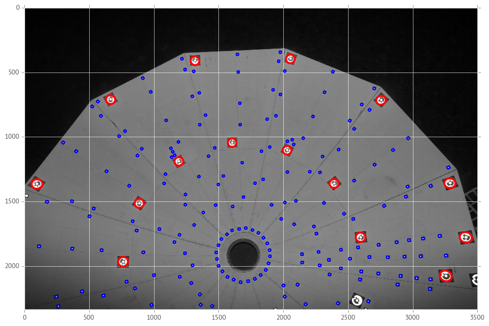
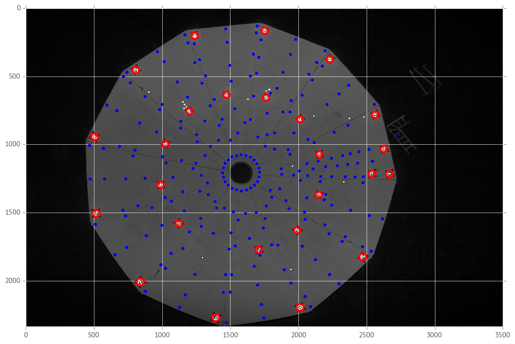
This is what I got:

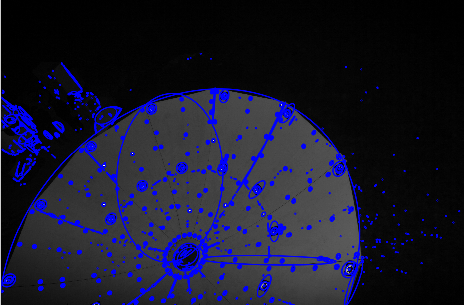
Every blue blob in that image is an ellipse. See a closeup:

In the closeup it is clear that the ellipses on the targets are where they should be but there are some that are obviously out of place. In particular, each black square has an ellipse that basically touches its four corners and then there are some that are seemingly fitted on nothing. Remember, they were fitted onto contours that were derived from the threshold image and this is the original image I’m using for illustration.

I did one more thing.

See those black squares around the targets? Well, they are also found by the contour function and hence each gets an ellipse fitted to it, badly. opencv has a function that will find the best-fitting polygon approximation for a contour, and I used this function to find (most) of the squares. The code looks like this:

def find_square_contours(self, epsilon=0.1, min_area=200, max_area=4000):
    ''' Find the ones that is approximately square
    '''
    squares = []
    for cnt in self.contours:
        area = abs(cv2.contourArea(cnt))
        err = epsilon*cv2.arcLength(cnt, True)
        hull = cv2.convexHull(cnt)
        approx = cv2.approxPolyDP(hull, err, True)
        if len(approx) != 4:
            continue
        if area < min_area:
            continue
        if area > max_area:
            continue
        square = Square(approx)
        squares.append(square)
    return squares

So at this point I have a list of ellipses (center, major and minor axis and rotation angle) as well as a list of squares (I know the coordinates of their corners).

Upwards and onwards!

Selecting the targets

The next part deals with selecting the things on the image that are in fact targets. ²

If you give the zoomed image of the ellipse fits a look, you’ll see that the ellipses that have been fit to each of them forms a kind of pattern. In the case of the larger RAD targets, there is an ellipse fitted around the central circle, another one on the outside of the outer ring and possibly one in between those two. In the case of the smaller uncoded targets, we usually see two ellipses: one around the target center and one fitted to the black square.

The next part of the algorithm chooses one of these types or discards both, for each ellipse and it does so in the following manner:

For each ellipse:

1. Calculate the encoding of a concentric ellipse that is 85% the size of the given ellipse.
2. Calculate the encoding of another concentric ellipse that is 60% the size of the ellipse.

If the first one has an encoding of ‘0111111111’ and the second has an encoding that starts with ‘0’ then I deem that ellipse as a RAD target.

For the small targets, the algorithm was a bit simpler. I made a list of the contours have have 4 corners (I used the aproxPoly function in opencv, which isn’t foolproof). I assumed these would mostly be the black squares around all the targets, but some of them may be spurious. For each of these polygons I calculated the length of the long and short sides. The selection for small targets worked as follows:

For each polygon:

1. Check if an ellipse falls inside.
2. Check if that ellipse is smaller than BOTH the long and short sides

If 1 and 2 is true then the ellipse that falls inside is deemed a target. So I made a list of ellipses that is deemed small targets.

But now I ran into a problem. The RAD targets also have polygons around them and ellipses inside. I got around this problem by then checking in a radius around each RAD target for the existence of small targets. If any of them fell inside the RAD target’s ellipse, I removed them from the small target list.

These algorithms can probably be improved and I’ll likely come back to them.

Next up, how I measured the encoding then the results.

Measuring the encoding of a target

Here’s what a RAD target looks like:

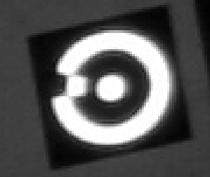
It looks a bit pixelated because it IS. This is what we get on a typical image. The idea is to work out some way of assigning a unique value to this RAD target, based on the markings that appears on it. In this particular example you can see the outer ring has a notch at about 9 o’clock. This signifies the zero angle or the ‘top’ of the target. So, for instance, we could rotate this image in such a way that the outer notch is at 12 o’clock, then look at which parts are coloured in and which are not. I decided to use a similar but slightly different method. It works as follows:

Let’s assume we are given the ellipse that falls on the outside edge of this target. Now let’s draw two smaller ellipses that is concentric to the outer ellipse, onto the target. Something like this:

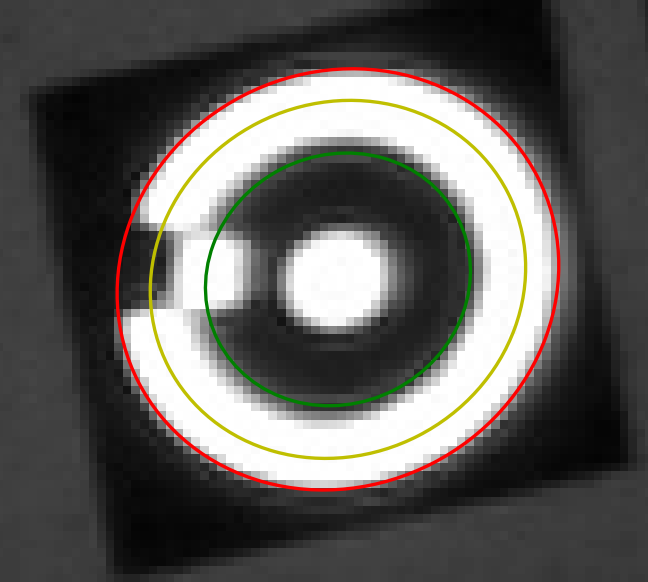
The middle (yellow) one is 85% the size of the outer (red) ellipse and the inner (green) ellipse is 60%. The next thing I did was to calculate the value of the threshold image along the perimeter of each of these ellipses. I get something like this:

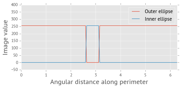
On the plot³ above you can see where the notches for both the inner and outer ellipses fall. They occur at the same distance along the perimeter of each ellipse but have opposite values. So now I can calculate how far I have to ‘rotate’ the perimeter values for the inner ellipse such that the filled notch is at the beginning of the perimeter, as calculated on this plot. This plot looks as follows once I’ve done that:

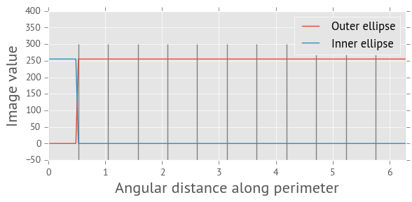
I’ve also marked the 12 segments along the inner perimeter with vertical lines. Calculating the encoding is now as simple as checking the ‘median’ value (or even the mode) of the values inside each segment. If it is 255, the value is 1 and zero if the median is 0. That way you can build up a string of 12 ones and zeros that uniquely identifies this target. WIN!

I’ve done something slightly different with the small targets and I may be able to use this algorithm on them too, in future. Something to try!

Putting it all together!

All that is left now is to show how well (and sometimes not so well) this method has worked. In the images below, the red ellipses denote RAD targets found and the blue ellipses are unencoded targets found.

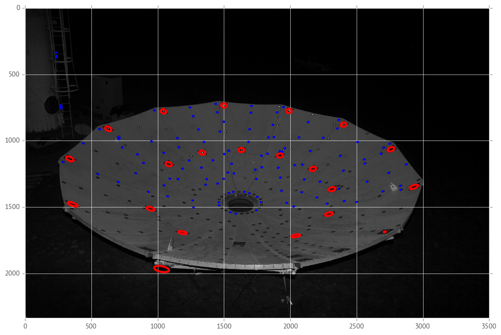
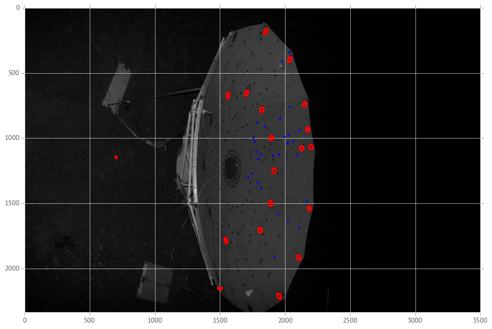
While looking at these, it becomes clear that the RAD-finding algorithm is fairly robust. It found most of the RAD targets even on the very oblique and poorly illuminated parts of the dish. The problem came in with the small targets. I know the reason is mainly because I used the black squares to search for them and the opencv function I used to count the number of corners didn’t pick up the oblique squares as having 4 corners. For both kinds of targets there are some spurious ones that are obviously (to the eye) not real.

I’ll be able to discard more of these spurious targets when I do the bundle adjustment since I’ll only be able to use those targets which occur on multiple images. More on that in future posts.

In the next post I’m going to do some MATHS! (if I can remember how to O_o)

It’ll be fun…